In web applications it’s very common to try to limit the results by group. For example showing all the new posts with the the two latest comments on them. Or have the best selling categories in an e-commerce website showing the 3 most popular products in those categories.
In MySQL you only have one option to iterate through your parent model (Post, Category) and do a query for every subsequent parent. This may or may not be what you want. If you have a large system you can even run them parallel and merge the results in the application which might lead to better overall query time but it costs you complexity and more resources being used concurrently making the database reaching its limits sooner.
In PostgreSQL you can do that in a single query. And actually two very different ways. Window functions are there for quite some time by now in PG and since 9.3 LATERAL JOINs are also available. Both enables us to get the results in a single query very efficiently. And we will also see how they compare in terms of performance.
Using window function
Prior to lateral joins this was the only option to have the limit per group functionality so it became sort of a de fact default for it.
|
1 2 3 4 5 6 7 8 |
select * from ( select *, row_number() over (partition by category_id order by popularity desc) as rownum from product p join category c on c.id = p.category_id where p.public and c.id IN (1, 2, 3, 4) ) a where rownum <= 3 order by category_id; |
It’s pretty simple once you get familiar with the syntax of window functions. It works the same way how we use group by but here we use partition by and gather the extra information row_number() which we can use in an outer query to filter out results.
Using LATERAL JOIN
|
1 2 3 4 5 6 7 8 9 |
select * from category join lateral ( select * from product where public and category_id = category.id order by popularity desc limit 3 ) p on true where category.id IN (1, 2, 3, 4) order by category.id; |
The lateral join enables us to refer the outer query’s tables in the joined subselect which makes it a very powerful tool. It is a bit easier to understand and gives a bit of more flexibility with the joins comparing to the previous example.
But which one runs faster?
Benchmark
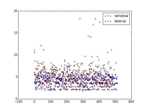
I will run the queries on a sample database with ~14000 products and ~350 categories first querying for random categories than for the largest ones only.
Random run
| AVG | Std dev | Min | Max | |
| Window | 5,197 ms | 2,059 ms | 2,562 ms | 18,273 ms |
| Lateral | 4,223 ms | 1,358 ms | 1,866 ms | 10,528 ms |
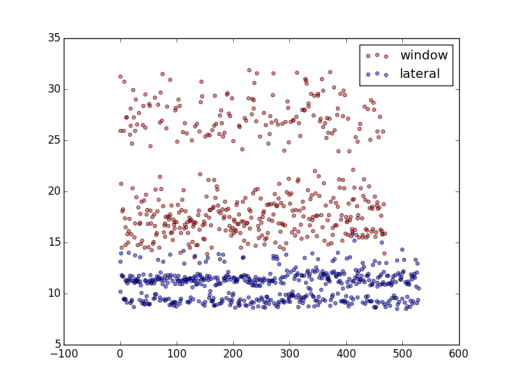
Large categories only
| AVG | Std dev | Min | Max | |
| Window | 20,746 ms | 5,114 ms | 13,535 ms | 31,894 ms |
| Lateral | 10,813 ms | 1,392 ms | 8,495 ms | 15,875 ms |
Conclusion
The results are not so surprising looking at the product distribution in the top 10 categories which shows that some categories are stuffed while the others have at least an order of magnitude less products.
|
1 2 3 4 5 6 7 8 9 10 11 12 13 14 |
+---------+ | count | |---------| | 7854 | | 1058 | | 356 | | 327 | | 248 | | 222 | | 180 | | 172 | | 126 | | 123 | +---------+ |
Querying the large categories obviously takes longer times but the impact is much more noticeable using the window functions because it actually has to fetch every row in the categories mark them with the row number and only filter that in the outer query while the lateral join limits the results for every category.
Are there any other ways to have the same results? Feel free to comment if you have further ideas to benchmark.


Recent comments